S1-S5 breast cancer contour application

This advanced pyXenium.contour tutorial uses the Atera Xenium WTA FFPE breast cancer export at Y:\long\10X_datasets\Xenium\Atera\WTA_Preview_FFPE_Breast_Cancer_outs to build five HistoSeg-backed contour annotations and then run contour-native biology and topology analyses.

The five annotation classes are intentionally broader than the basic contour tutorial:

S class	Biological compartment	Aggregated Atera cell groups
S1	Invasive tumor plus invasion-associated CAFs	CAFs Invasive Associated, 11q13 invasive tumor, G1/S, mitotic
S2	Basal-like structured DCIS plus lymphoid/DC	Basal DCIS, dendritic cells, B cells, T lymphocytes
S3	Myeloid-vascular-stromal niche	Mast/myeloid/macrophage, CXCL14+ fibroblast, endothelial, pericyte
S4	Myoepithelial/DCIS CAF/plasma compartment	Myoepithelial, DCIS-associated CAFs, plasma cells
S5	Apocrine/luminal amorphous DCIS axis	Apocrine and luminal-like amorphous DCIS

The committed RTD snapshot is generated from a whole-transcriptome transcript scan. The lightweight tables below are top slices from the all-gene results; no curated DEG panel is used for gene selection.

from __future__ import annotations

from pathlib import Path
import json
import shutil
import sys

import matplotlib.pyplot as plt
import numpy as np
import pandas as pd
import seaborn as sns
from IPython.display import Markdown, display


def _find_repo_root() -> Path:
    cwd = Path.cwd().resolve()
    for candidate in (cwd, *cwd.parents):
        if (candidate / 'src' / 'pyXenium').exists():
            return candidate
    return cwd

PROJECT_ROOT = _find_repo_root()
SRC_ROOT = PROJECT_ROOT / 'src'
if str(SRC_ROOT) not in sys.path:
    sys.path.insert(0, str(SRC_ROOT))

from pyXenium.contour import (
    add_contours_from_geojson,
    compare_contour_cell_composition,
    compare_contour_transcript_de,
    generate_barrier_contour_shells,
    generate_xenium_explorer_annotations,
)
from pyXenium.io import XeniumFrameChunkSource, read_xenium
from pyXenium.io.api import TRANSCRIPT_POINT_COLUMNS, TRANSCRIPT_POINT_COLUMN_TYPES
from pyXenium.io.xenium_artifacts import iter_transcript_chunks

sns.set_theme(context='notebook', style='whitegrid')

DATASET_ROOT = Path(r'Y:\long\10X_datasets\Xenium\Atera\WTA_Preview_FFPE_Breast_Cancer_outs')
HISTOSEG_ROOT = Path(r'D:\GitHub\HistoSeg')
OUTPUT_ROOT = DATASET_ROOT / 'pyxenium_tutorial_outputs' / 'atera_s1_s5_contour_application'
FIGURE_DIR = OUTPUT_ROOT / 'figures'
STATIC_SNAPSHOT_DIR = PROJECT_ROOT / 'docs' / '_static' / 'tutorials' / 'contour_s1_s5'
GRAPHCLUST_RELPATH = Path('analysis/analysis/clustering/gene_expression_graphclust/clusters.csv')
CELL_GROUPS_PATH = DATASET_ROOT / 'WTA_Preview_FFPE_Breast_Cancer_cell_groups.csv'
CELLS_PARQUET_RELPATH = Path('cells.parquet')
TRANSCRIPTS_PATH = DATASET_ROOT / 'transcripts.parquet'
S1_S5_GEOJSON = DATASET_ROOT / 'xenium_explorer_annotations.s1_s5.generated.geojson'
PIXEL_SIZE_UM = 0.2125
QUALITY_QUERY = 'quality_score >= 20 and valid == True'

RUN_HISTOSEG_EXPORT = False
RUN_TRANSCRIPT_SNAPSHOT = False

OUTPUT_ROOT.mkdir(parents=True, exist_ok=True)
FIGURE_DIR.mkdir(parents=True, exist_ok=True)
STATIC_SNAPSHOT_DIR.mkdir(parents=True, exist_ok=True)


def top_ok(frame: pd.DataFrame, n: int = 200) -> pd.DataFrame:
    local = frame.loc[frame.get('status', 'ok').eq('ok')].copy()
    if local.empty:
        local = frame.copy()
    return local.head(n).reset_index(drop=True)


def top_one_vs_rest_snapshot(frame: pd.DataFrame, per_case: int = 30) -> pd.DataFrame:
    local = frame.loc[frame.get('status', 'ok').eq('ok')].copy()
    if local.empty:
        local = frame.copy()
    return (
        local.sort_values(['case', 'fdr', 'p_value', 'gene'], na_position='last', kind='stable')
        .groupby('case', group_keys=False)
        .head(per_case)
        .reset_index(drop=True)
    )

1. Build the S1-S5 structure definitions

The official GraphClust table stores numeric cluster IDs, while the Atera cell-group CSV stores readable labels and colors. We bridge those tables and aggregate cluster IDs into the five S classes. Two user-facing names are aliased to the exact dataset labels: CAFs Invasive Associated -> CAFs, Invasive Associated and CAFs DCIS Associated -> CAFs, DCIS Associated.

S1_S5_PANEL = {
    'S1': [
        'CAFs Invasive Associated',
        '11q13 Invasive Tumor Cells',
        '11q13 Invasive Tumor Cells (G1/S)',
        '11q13 Invasive Tumor Cells (Mitotic)',
    ],
    'S2': [
        'Basal-like Structured DCIS Cells',
        'Dendritic Cells',
        'B Cells',
        'T Lymphocytes',
    ],
    'S3': [
        'Mast Cells',
        'Myeloid Cells',
        'Macrophages',
        'CXCL14+ Fibroblasts',
        'Endothelial Cells',
        'Pericytes',
    ],
    'S4': [
        'Myoepithelial Cells',
        'CAFs DCIS Associated',
        'Plasma Cells',
    ],
    'S5': [
        'Apocrine Cells',
        'Luminal-like Amorphous DCIS Cells',
    ],
}

LABEL_ALIASES = {
    'CAFs Invasive Associated': 'CAFs, Invasive Associated',
    'CAFs DCIS Associated': 'CAFs, DCIS Associated',
}
S_COLORS = {'S1': '#C43C39', 'S2': '#3F7CAC', 'S3': '#4A9D67', 'S4': '#B9802D', 'S5': '#9A5BC7'}
S_DESCRIPTIONS = {
    'S1': 'Invasive tumor + CAFs',
    'S2': 'Basal DCIS + lymphoid',
    'S3': 'Myeloid-vascular-stromal',
    'S4': 'Myoepithelial/DCIS CAF/plasma',
    'S5': 'Apocrine/luminal DCIS',
}

cluster_df = pd.read_csv(DATASET_ROOT / GRAPHCLUST_RELPATH)
cell_groups_df = pd.read_csv(CELL_GROUPS_PATH).rename(columns={'cell_id': 'Barcode', 'group': 'cell_group'})
cluster_bridge = cluster_df.merge(
    cell_groups_df[['Barcode', 'cell_group', 'color']],
    on='Barcode',
    how='inner',
)
label_to_clusters = (
    cluster_bridge.groupby('cell_group')['Cluster']
    .apply(lambda values: sorted(pd.Series(values).dropna().astype(int).unique().tolist()))
    .to_dict()
)
label_counts = cluster_bridge.groupby('cell_group').size().to_dict()

structures = []
structure_rows = []
for idx, (structure_name, requested_labels) in enumerate(S1_S5_PANEL.items(), start=1):
    cluster_ids = []
    resolved_labels = []
    input_cell_count = 0
    for requested_label in requested_labels:
        resolved_label = LABEL_ALIASES.get(requested_label, requested_label)
        if resolved_label not in label_to_clusters:
            raise KeyError(f'Missing Atera cell group: {requested_label!r} -> {resolved_label!r}')
        cluster_ids.extend(label_to_clusters[resolved_label])
        resolved_labels.append(resolved_label)
        input_cell_count += int(label_counts[resolved_label])

    structures.append(
        {
            'structure_name': structure_name,
            'cluster_ids': sorted(set(cluster_ids)),
            'structure_color': S_COLORS[structure_name],
            'structure_id': idx,
            'member_labels': tuple(resolved_labels),
        }
    )
    structure_rows.append(
        {
            'structure_name': structure_name,
            'description': S_DESCRIPTIONS[structure_name],
            'cluster_ids': sorted(set(cluster_ids)),
            'member_labels': ', '.join(resolved_labels),
            'input_cell_count': input_cell_count,
        }
    )

structure_definition_table = pd.DataFrame(structure_rows)
display(structure_definition_table)

2. Generate HistoSeg-backed Xenium Explorer annotations

generate_xenium_explorer_annotations(...) calls the HistoSeg multi-structure contour API and writes a Xenium Explorer-compatible GeoJSON. The legacy xenium_explorer_annotations.geojson is left untouched; this tutorial writes xenium_explorer_annotations.s1_s5.generated.geojson.

if RUN_HISTOSEG_EXPORT or not S1_S5_GEOJSON.exists():
    artifacts = generate_xenium_explorer_annotations(
        DATASET_ROOT,
        structures=structures,
        output_relpath=OUTPUT_ROOT.relative_to(DATASET_ROOT),
        clusters_relpath=GRAPHCLUST_RELPATH,
        cells_parquet_relpath=CELLS_PARQUET_RELPATH,
        histoseg_root=HISTOSEG_ROOT if HISTOSEG_ROOT.exists() else None,
        min_cells=500,
        min_component_pixels=180,
        xenium_pixel_size_um=PIXEL_SIZE_UM,
    )
    shutil.copy2(artifacts['geojson'], S1_S5_GEOJSON)
else:
    artifacts = {
        'geojson': str(S1_S5_GEOJSON),
        'out_dir': str(OUTPUT_ROOT),
        'preview_png': str(OUTPUT_ROOT / 'multi_structure_contour_preview.png'),
    }

contour_counts = pd.read_csv(OUTPUT_ROOT / 's1_s5_contour_counts.csv') if (OUTPUT_ROOT / 's1_s5_contour_counts.csv').exists() else pd.read_csv(OUTPUT_ROOT / 'structure_contour_cell_counts.csv')
display(contour_counts)
artifacts

Snapshot contour counts

The committed RTD snapshot includes this small result table, so the page remains informative even with notebook execution disabled.

structure_name	description	input_cell_count	assigned_cell_count	contour_count
S1	Invasive tumor + CAFs	72873	71725	106
S2	Basal DCIS + lymphoid	23298	15935	358
S3	Myeloid-vascular-stromal	26690	37038	491
S4	Myoepithelial/DCIS CAF/plasma	33753	36486	313
S5	Apocrine/luminal DCIS	13431	8861	28

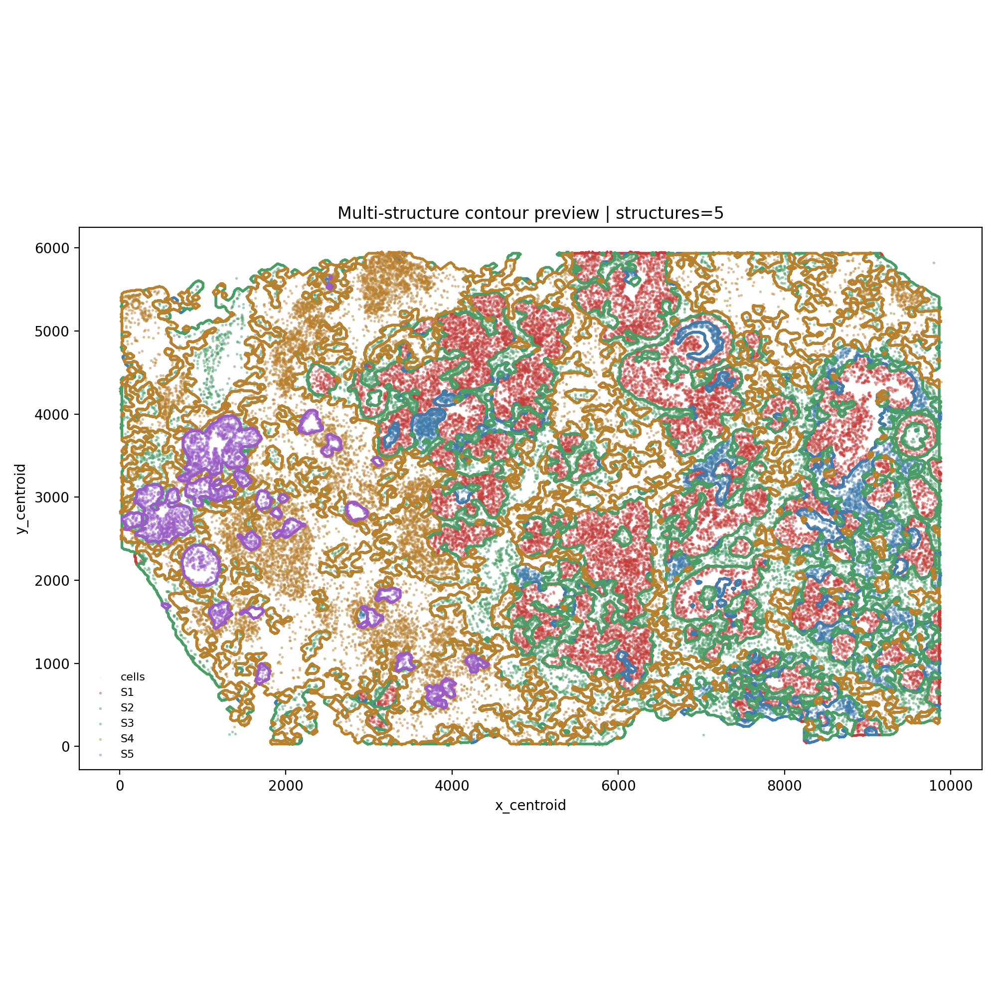
Annotation preview

The generated S1-S5 export contains multiple contours per class. In the snapshot run, the HistoSeg count table reported 106 S1, 358 S2, 491 S3, 313 S4, and 28 S5 contour components before GeoJSON polygon serialization.

3. Load Xenium, import contours, and attach cell-group labels

We load the cell table without materializing the full transcript parquet. When RUN_TRANSCRIPT_SNAPSHOT=True, the notebook attaches the unfiltered transcripts.parquet stream and lets compare_contour_transcript_de(..., genes=None) discover all genes from the whole transcriptome. The RTD page keeps execution off and displays the committed whole-transcriptome snapshot tables and figures.

slide = read_xenium(
    str(DATASET_ROOT),
    as_='slide',
    include_transcripts=False,
    include_boundaries=False,
    include_images=False,
    clusters_relpath=str(GRAPHCLUST_RELPATH),
)
cell_group_map = cell_groups_df.set_index('Barcode')['cell_group']
slide.table.obs['cell_group'] = slide.table.obs.index.map(cell_group_map).fillna('Unassigned')

add_contours_from_geojson(
    slide,
    S1_S5_GEOJSON,
    key='s1_s5_contours',
    id_key='name',
    pixel_size_um=PIXEL_SIZE_UM,
)

print(slide.component_summary())
print(sorted(slide.shapes['s1_s5_contours']['assigned_structure'].dropna().unique()))

def attach_whole_transcript_source(slide, genes=None) -> None:
    gene_filter = None if genes is None else set(str(gene) for gene in genes)
    slide.points.pop('transcripts', None)
    slide.point_sources['transcripts'] = XeniumFrameChunkSource(
        columns=TRANSCRIPT_POINT_COLUMNS,
        column_types=TRANSCRIPT_POINT_COLUMN_TYPES,
        chunk_iter_factory=lambda: iter_transcript_chunks(str(TRANSCRIPTS_PATH), genes=gene_filter),
        attrs={
            'source_path': str(TRANSCRIPTS_PATH),
            'gene_filter': None if gene_filter is None else tuple(sorted(gene_filter)),
            'analysis_mode': 'whole_transcriptome',
        },
        preserve_extra_columns=True,
    )


if RUN_TRANSCRIPT_SNAPSHOT:
    attach_whole_transcript_source(slide)

4. Transcript-level contour DEG

compare_contour_transcript_de(...) aggregates raw transcript counts into contour-level pseudobulks, computes contour-level CPM/log1p CPM, and treats each contour as a replicate. Here genes=None means the DEG scan is whole-transcriptome: every gene observed in the unfiltered transcript stream is tested before the top snapshot rows are selected for RTD. For this whole-transcriptome screening step, assignment='cell_id' uses the cell_id field in transcripts.parquet and assigns cell-associated transcripts through the contour membership of each cell centroid, which is much faster than point-in-polygon testing 740M transcript coordinates.

if RUN_TRANSCRIPT_SNAPSHOT:
    deg_result_full = compare_contour_transcript_de(
        slide,
        contour_key='s1_s5_contours',
        groupby='assigned_structure',
        genes=None,
        assignment='cell_id',
        comparisons=('global', 'one_vs_rest'),
        transcript_query=QUALITY_QUERY,
        min_total_transcripts_per_contour=1,
        min_contours_per_group=2,
        include_zero_counts=False,
        return_contour_gene=False,
    )
    deg_result_full['global_de'].to_csv(
        OUTPUT_ROOT / 's1_s5_transcript_de_global.whole_transcriptome.full.csv', index=False
    )
    deg_result_full['one_vs_rest_de'].to_csv(
        OUTPUT_ROOT / 's1_s5_transcript_de_one_vs_rest.whole_transcriptome.full.csv', index=False
    )
    deg_result = {
        'global_de': top_ok(deg_result_full['global_de'], 200),
        'one_vs_rest_de': top_one_vs_rest_snapshot(deg_result_full['one_vs_rest_de'], per_case=30),
    }
    deg_result['global_de'].to_csv(OUTPUT_ROOT / 's1_s5_transcript_de_global.csv', index=False)
    deg_result['one_vs_rest_de'].to_csv(OUTPUT_ROOT / 's1_s5_transcript_de_one_vs_rest.csv', index=False)
else:
    deg_result = {
        'global_de': pd.read_csv(STATIC_SNAPSHOT_DIR / 's1_s5_transcript_de_global.csv'),
        'one_vs_rest_de': pd.read_csv(STATIC_SNAPSHOT_DIR / 's1_s5_transcript_de_one_vs_rest.csv'),
    }

display(deg_result['global_de'].head(12))
display(deg_result['one_vs_rest_de'].head(12))

Snapshot DEG tables

Top global genes from the whole-transcriptome contour-level Kruskal-Wallis test. These rows are a committed top slice from 18,028 tested genes, not a curated panel.

gene	top_group	bottom_group	delta_log1p_cpm	delta_mean_density_per_um2	fdr
EGFL7	S3	S4	3.47	0.00167	6.01e-88
SHANK3	S3	S4	3.17	0.00148	2.48e-73
EPAS1	S3	S2	3.08	0.004026	2.48e-73
CD36	S3	S4	3.35	0.00161	3.09e-73
VWF	S3	S4	3.48	0.003595	2.02e-71
KDR	S3	S4	3.01	0.001556	9.05e-67
CDH5	S3	S2	2.77	0.0009097	1.02e-64
PECAM1	S3	S4	3.16	0.002475	8.99e-64

Top two one-vs-rest whole-transcriptome genes per S class:

case	gene	log2fc_cpm	fdr
S1	SPATA20	1.71	5.98e-36
S1	SLC35F5	0.68	2.03e-33
S2	EGFL7	-2.44	9.62e-37
S2	PDE2A	-3.19	4.2e-36
S3	CD36	2.6	3.62e-82
S3	EGFL7	2.97	4.46e-78
S4	PCDH17	-2.64	4.86e-32
S4	SHANK3	-2.11	7.78e-30
S5	GRHL2	1.83	1.73e-175
S5	VWA2	1.77	2.61e-156

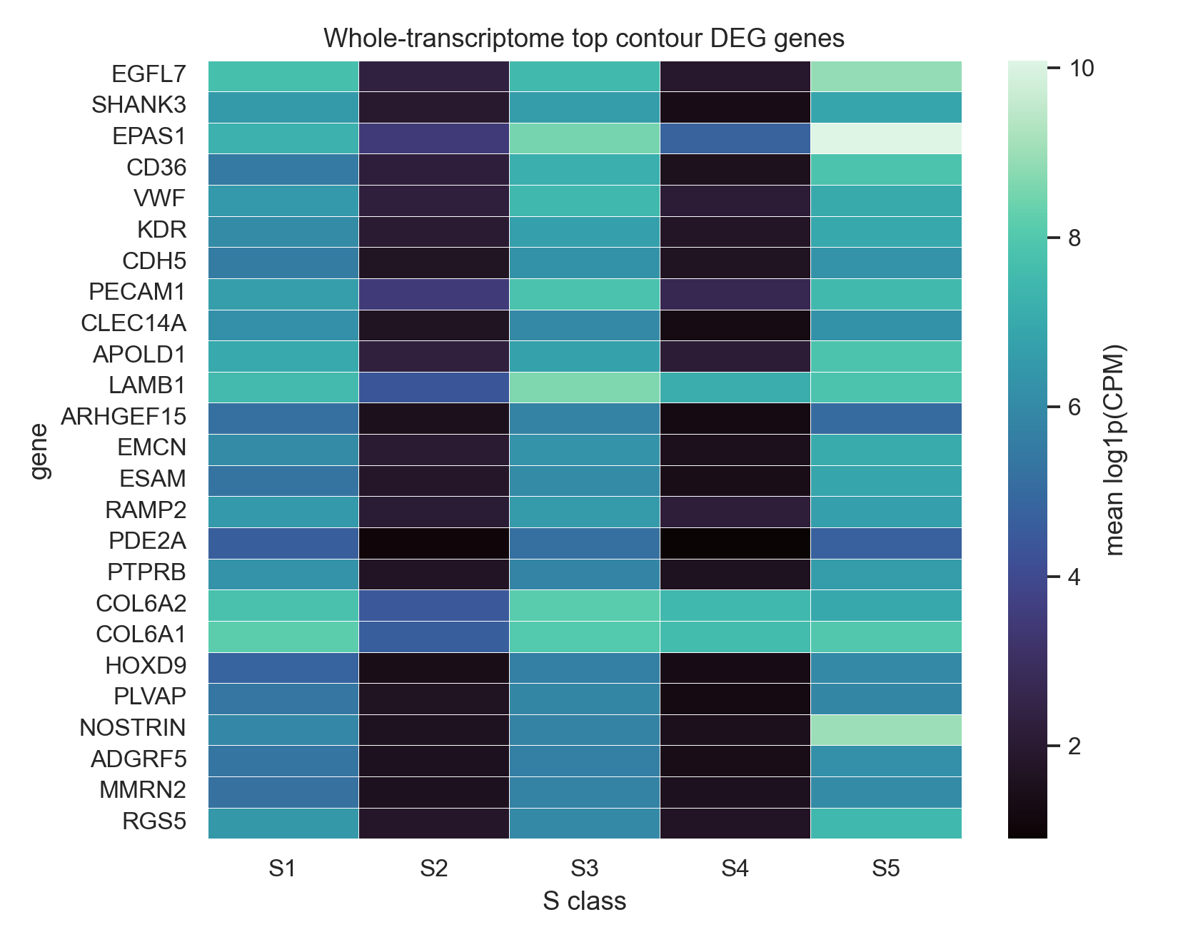
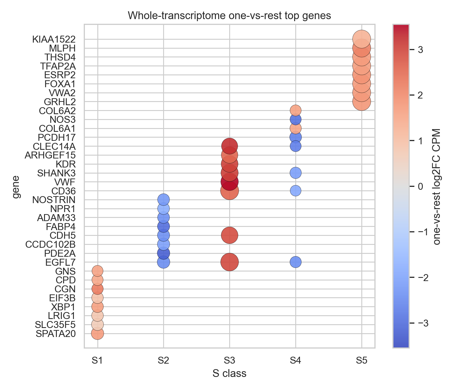
DEG visualization

The heatmap shows mean contour-level log1p(CPM) for top genes selected from the whole-transcriptome global test. The dotplot summarizes the strongest whole-transcriptome one-vs-rest signals per S class.

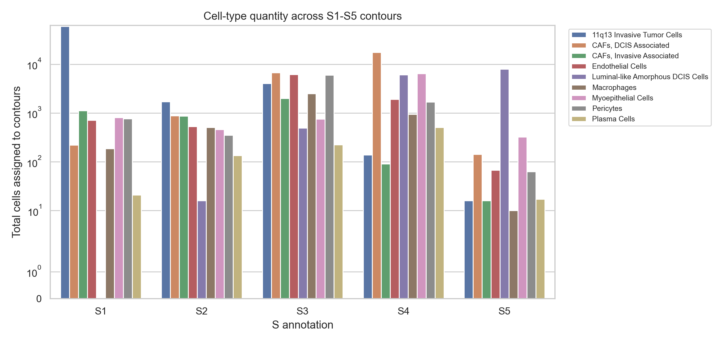
5. Cell-type composition across contour classes

compare_contour_cell_composition(...) assigns cell centroids to every contour independently. It reports both proportions and quantities, then tests S-class differences with Kruskal-Wallis globally and Mann-Whitney tests pairwise.

if RUN_TRANSCRIPT_SNAPSHOT:
    cell_result = compare_contour_cell_composition(
        slide,
        contour_key='s1_s5_contours',
        groupby='assigned_structure',
        cell_type_key='cell_group',
    )
    cell_result['group_summary'].to_csv(OUTPUT_ROOT / 's1_s5_cell_composition_group_summary.csv', index=False)
    pd.concat(
        [
            cell_result['global_stats'].assign(test_scope='global'),
            cell_result['pairwise_stats'].assign(test_scope='pairwise'),
        ],
        ignore_index=True,
        sort=False,
    ).to_csv(OUTPUT_ROOT / 's1_s5_cell_composition_stats.csv', index=False)
else:
    cell_result = {
        'group_summary': pd.read_csv(STATIC_SNAPSHOT_DIR / 's1_s5_cell_composition_group_summary.csv'),
        'stats': pd.read_csv(STATIC_SNAPSHOT_DIR / 's1_s5_cell_composition_stats.csv'),
    }

display(cell_result['group_summary'].head(12))
if 'stats' in cell_result:
    display(cell_result['stats'].head(12))

Snapshot cell-composition statistics

Top global cell-type composition differences across S1-S5 contours:

cell_type	metric	top_group	bottom_group	fdr
Pericytes	n_cells	S3	S2	6.01e-98
Endothelial Cells	n_cells	S3	S2	1.40e-94
Pericytes	fraction	S3	S5	3.49e-90
Endothelial Cells	fraction	S3	S1	1.06e-89
Luminal-like Amorphous DCIS Cells	n_cells	S5	S1	5.84e-77
CXCL14+ Fibroblasts	n_cells	S1	S2	5.35e-76
CAFs, DCIS Associated	fraction	S4	S1	7.76e-70
Luminal-like Amorphous DCIS Cells	fraction	S5	S1	2.62e-67

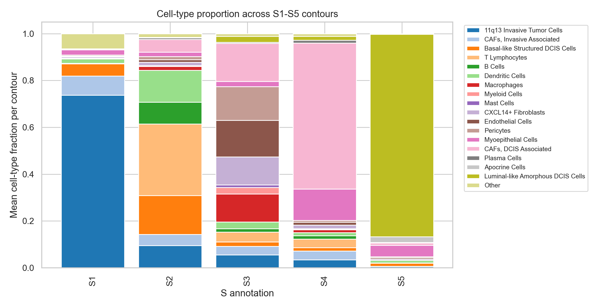
Composition visualization

6. Barrier-aware S1/S4/S5 boundary shells

The boundary question asks how S1, S4, and S5 contours behave when expanded inward and outward in 20 um steps. We generate 10 signed rings: [-100,-80] ... [-20,0] and [0,20] ... [80,100]. Outward rings are clipped by all other S1-S5 contour interiors, so a shell stops contributing when it reaches another annotated contour.

selected_frame = slide.shapes['s1_s5_contours'].loc[
    slide.shapes['s1_s5_contours']['assigned_structure'].isin(['S1', 'S4', 'S5'])
].copy()
slide.shapes['s1_s4_s5_contours'] = selected_frame
slide.metadata.setdefault('contours', {})['s1_s4_s5_contours'] = {
    'units': 'micron',
    'derived_from_key': 's1_s5_contours',
}

if 's1_s4_s5_barrier_shells' not in slide.shapes:
    generate_barrier_contour_shells(
        slide,
        contour_key='s1_s4_s5_contours',
        barrier_contour_key='s1_s5_contours',
        inward=100.0,
        outward=100.0,
        step_size=20.0,
        output_key='s1_s4_s5_barrier_shells',
    )

shell_frame = slide.shapes['s1_s4_s5_barrier_shells']
slide.shapes['s1_s4_s5_boundary_outward_0_60'] = shell_frame.loc[
    shell_frame['shell_direction'].eq('outward')
    & (shell_frame['shell_start'] >= 0)
    & (shell_frame['shell_end'] <= 60)
].copy()
slide.metadata.setdefault('contours', {})['s1_s4_s5_boundary_outward_0_60'] = {
    'units': 'micron',
    'derived_from_key': 's1_s4_s5_barrier_shells',
}

display(shell_frame[['contour_id', 'source_contour_id', 'assigned_structure', 'shell_start', 'shell_end', 'shell_direction']].head())
print('shell contours:', shell_frame['contour_id'].nunique())
print('outward 0-60 um shells:', slide.shapes['s1_s4_s5_boundary_outward_0_60']['contour_id'].nunique())

if RUN_TRANSCRIPT_SNAPSHOT:
    boundary_result_full = compare_contour_transcript_de(
        slide,
        contour_key='s1_s4_s5_boundary_outward_0_60',
        groupby='assigned_structure',
        genes=None,
        assignment='cell_id',
        comparisons=('global',),
        transcript_query=QUALITY_QUERY,
        min_total_transcripts_per_contour=0,
        min_contours_per_group=2,
        include_zero_counts=False,
        return_contour_gene=False,
    )
    boundary_stats = top_ok(boundary_result_full['global_de'], 200)
    boundary_result_full['global_de'].to_csv(
        OUTPUT_ROOT / 's1_s4_s5_boundary_de_global_outward_0_60.whole_transcriptome.full.csv', index=False
    )
    boundary_stats.to_csv(OUTPUT_ROOT / 's1_s4_s5_boundary_de_global_outward_0_60.csv', index=False)

    top_boundary_genes = boundary_stats['gene'].head(10).tolist()
    attach_whole_transcript_source(slide, genes=top_boundary_genes)
    shell_result = compare_contour_transcript_de(
        slide,
        contour_key='s1_s4_s5_barrier_shells',
        groupby='assigned_structure',
        genes=top_boundary_genes,
        comparisons=('global',),
        transcript_query=QUALITY_QUERY,
        min_total_transcripts_per_contour=0,
        min_contours_per_group=2,
        include_zero_counts=True,
        return_contour_gene=True,
    )
    shell_gene = shell_result['contour_gene'].copy()
    boundary_curves = (
        shell_gene.loc[shell_gene['gene'].isin(top_boundary_genes)]
        .groupby(['assigned_structure', 'gene', 'shell_start', 'shell_end', 'shell_mid'], as_index=False)
        .agg(
            mean_density_per_um2=('density_per_um2', 'mean'),
            sem_density_per_um2=('density_per_um2', lambda values: float(pd.Series(values).sem())),
            n_shells=('contour_id', 'nunique'),
            total_count=('count', 'sum'),
        )
        .sort_values(['gene', 'assigned_structure', 'shell_mid'], kind='stable')
    )
    boundary_curves.to_csv(OUTPUT_ROOT / 's1_s4_s5_barrier_ring_density_top10.csv', index=False)
else:
    boundary_curves = pd.read_csv(STATIC_SNAPSHOT_DIR / 's1_s4_s5_barrier_ring_density_top10.csv')
    boundary_stats = pd.read_csv(STATIC_SNAPSHOT_DIR / 's1_s4_s5_boundary_de_global_outward_0_60.csv')

display(boundary_stats.head(10))
display(boundary_curves.head(10))

Snapshot boundary DE table

Top boundary genes were selected from a whole-transcriptome DEG scan on outward 0-60 um barrier-clipped shells. The screening step uses cell-associated transcripts assigned by cell centroid for scalability; the density curves below re-count these top genes from transcript coordinates across all 10 signed-distance steps.

gene	top_group	bottom_group	delta_log1p_cpm	delta_mean_density_per_um2	fdr
SLC39A6	S1	S4	1.48	0.00204	2.81e-21
AGR3	S1	S4	1.56	0.003781	2.81e-21
CERS2	S1	S4	1.57	0.001149	2.81e-21
TPBG	S1	S5	1.07	0.0009283	2.81e-21
TJP1	S1	S4	1.16	0.0006458	2.91e-21
ELAPOR1	S1	S4	1.65	0.002875	2.98e-21
DDB1	S1	S4	1.53	0.001435	4.46e-21
GNS	S5	S4	2.03	0.01711	4.49e-21
TNFSF10	S1	S4	1.68	0.004175	4.49e-21
SPATA20	S1	S4	1.52	0.002	5.14e-21

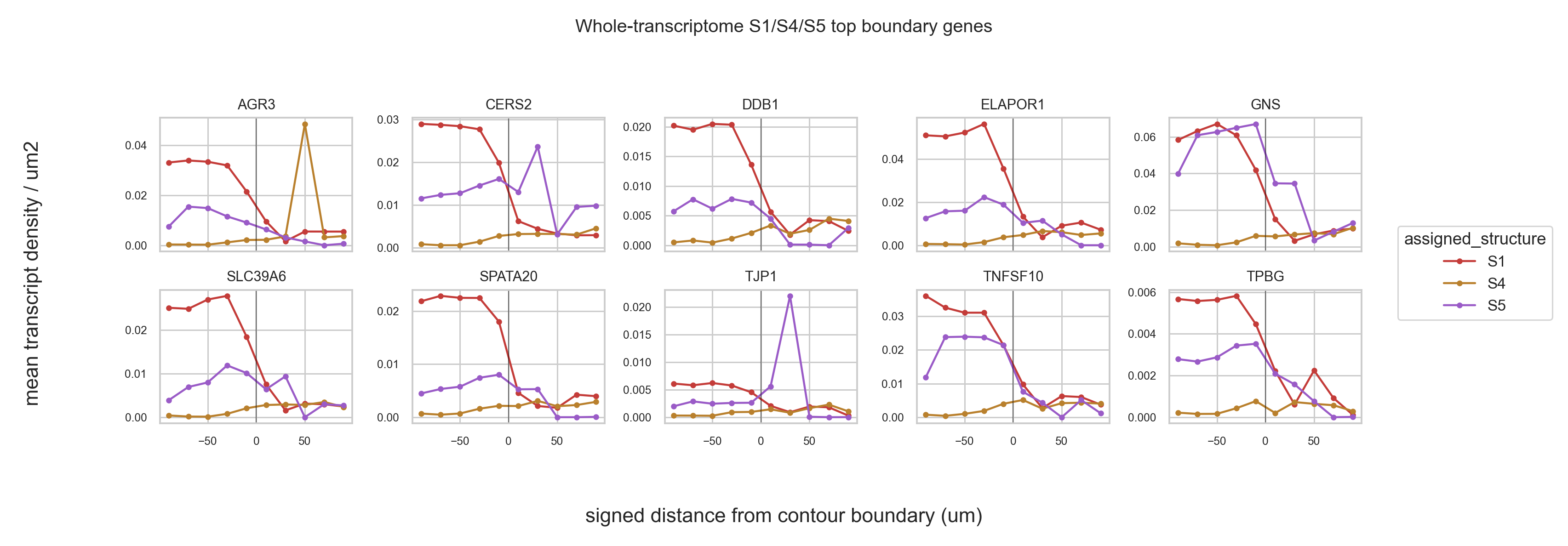
Boundary density curves

Top boundary genes were selected from a whole-transcriptome DEG scan on cell-associated transcripts whose cell centroids fall in the outward 0-60 um barrier-clipped shells. After those top genes are selected, their density curves are re-counted from transcript coordinates across the full 10 signed-distance steps. Negative distances are inside the source contour; positive distances are outside but barrier-clipped so they do not enter another contour.

7. Biological interpretation

The S1-S5 contours recover expected compartment-level organization, but the whole-transcriptome scan also makes the dominant axes more explicit than the earlier marker-panel snapshot.

• S1 remains an invasive tumor/CAF-rich compartment. Its one-vs-rest top genes include SPATA20, SLC35F5, LRIG1, XBP1, CGN, CPD, GNS, and ANXA2, consistent with an epithelial tumor program mixed with stress/secretory and invasion-associated biology.

• S2 is a basal-like structured DCIS plus lymphoid/DC compartment. In the whole-transcriptome one-vs-rest table, its strongest contrasts are largely negative vascular/endothelial genes such as EGFL7, PDE2A, CCDC102B, CDH5, and FABP4, supporting that S2 is less vascular than the S3/S5-rich microenvironments.

• S3 is the clearest vascular-stromal niche. The global top genes are dominated by endothelial/perivascular markers, including EGFL7, EPAS1, VWF, KDR, CDH5, PECAM1, CLEC14A, EMCN, ESAM, RAMP2, PTPRB, PLVAP, MMRN2, and RGS5.

• S4 combines myoepithelial cells, DCIS-associated CAFs, and plasma cells. Its strongest one-vs-rest contrasts include matrix-associated COL6A1 and COL6A2, while several endothelial genes are lower than the rest, separating it from the S3 vascular niche.

• S5 is the luminal/apocrine DCIS axis. Its one-vs-rest top genes include epithelial/luminal regulatory and differentiation genes such as MLPH, TFAP2A, ESRP2, FOXA1, GRHL2, and VWA2.

• For S1/S4/S5 boundary ecology, whole-transcriptome outward 0-60 um screening selected SLC39A6, AGR3, CERS2, TPBG, TJP1, ELAPOR1, DDB1, GNS, TNFSF10, and SPATA20. Coordinate-based density curves show many of these genes are highest inside S1 and/or S5 and decline across the boundary, which supports an epithelial/luminal boundary program rather than a purely stromal outward signal.

A practical analysis pattern emerges: use whole-transcriptome compare_contour_transcript_de to identify contour-level programs, compare_contour_cell_composition to explain which cell types make those programs plausible, and generate_barrier_contour_shells plus coordinate-counted transcript density curves to test whether a program sits inside the contour, peaks at the boundary, or extends into the surrounding microenvironment.

8. Contour adjacency network analysis

HistoSeg also provides a contour adjacency network layer. Here we reuse the already imported S1-S5 contour geometries, aggregate pairwise boundary-neighbor and enclosure relationships by assigned_structure, and render a compact network/heatmap snapshot for RTD. The adjacency score combines shared border length with enclosure-derived inner contour perimeter, so it captures both geography-like border contact and one compartment wrapping around another.

histoseg_src = HISTOSEG_ROOT / 'src'
if histoseg_src.exists() and str(histoseg_src) not in sys.path:
    sys.path.insert(0, str(histoseg_src))

from histoseg.contour import ContourAdjacencyConfig, run_contour_adjacency
from pyXenium.contour._geometry import contour_frame_to_geometry_table

ADJACENCY_ROOT = OUTPUT_ROOT / 's1_s5_contour_adjacency'
ADJACENCY_ROOT.mkdir(parents=True, exist_ok=True)

adjacency_contours = contour_frame_to_geometry_table(
    slide.shapes['s1_s5_contours'],
    contour_key='s1_s5_contours',
)[['contour_id', 'assigned_structure', 'classification_name', 'structure_id', 'geometry']].copy()
adjacency_contours = adjacency_contours.rename(columns={'assigned_structure': 'structure'})

adjacency_result = run_contour_adjacency(
    ContourAdjacencyConfig(
        contours=adjacency_contours,
        out_dir=ADJACENCY_ROOT,
        groupby='structure',
        contour_id_col='contour_id',
        geometry_col='geometry',
        boundary_tolerance=1.0,
        min_shared_boundary=0.0,
        enclosure_min_fraction=0.95,
        dpi=220,
        save_preview_png=True,
    )
)

adjacency_edges = pd.read_csv(adjacency_result.edges_csv)
adjacency_matrix = pd.read_csv(adjacency_result.matrix_csv, index_col=0)

snapshot_files = {
    adjacency_result.edges_csv: STATIC_SNAPSHOT_DIR / 's1_s5_contour_adjacency_edges.csv',
    adjacency_result.matrix_csv: STATIC_SNAPSHOT_DIR / 's1_s5_contour_adjacency_matrix.csv',
    adjacency_result.network_png: STATIC_SNAPSHOT_DIR / 's1_s5_contour_adjacency_network.png',
    adjacency_result.heatmap_png: STATIC_SNAPSHOT_DIR / 's1_s5_contour_adjacency_heatmap.png',
    adjacency_result.combined_png: STATIC_SNAPSHOT_DIR / 's1_s5_contour_adjacency_overview.png',
}
for src, dst in snapshot_files.items():
    if src is not None:
        shutil.copy2(src, dst)

display(adjacency_edges.sort_values('total_adjacency_length_um', ascending=False).head(10))
display(adjacency_matrix)
adjacency_result

Snapshot adjacency edge table

The committed RTD snapshot below was generated with HistoSeg cca55df using boundary_tolerance=1.0 um and enclosure_min_fraction=0.95. It summarizes 1578 S1-S5 contours into 10 cross-structure group pairs; 9 pairs have non-zero adjacency.

group_a	group_b	boundary_pair_count	boundary_shared_length_um	enclosure_pair_count	enclosure_inner_boundary_length_um	total_adjacency_length_um
S3	S4	557	169686	133	80123	249809
S1	S3	323	101744	24	14576.8	116321
S2	S3	672	61709.2	17	2671.4	64380.6
S1	S2	319	33515.6	25	8347.4	41863
S2	S4	374	20373.1	38	4923	25296.1
S4	S5	43	6750.1	15	9422.4	16172.5
S1	S4	163	10859.2	1	61.1	10920.2
S3	S5	75	10650.1	1	266.9	10917
S2	S5	12	554.3	0	0	554.3

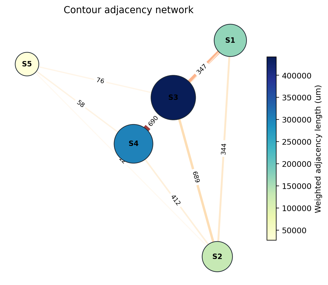
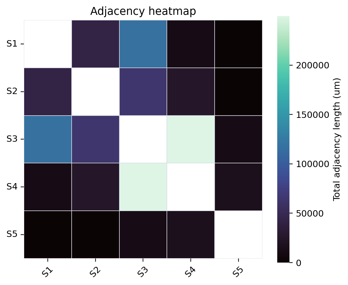
Adjacency network and heatmap

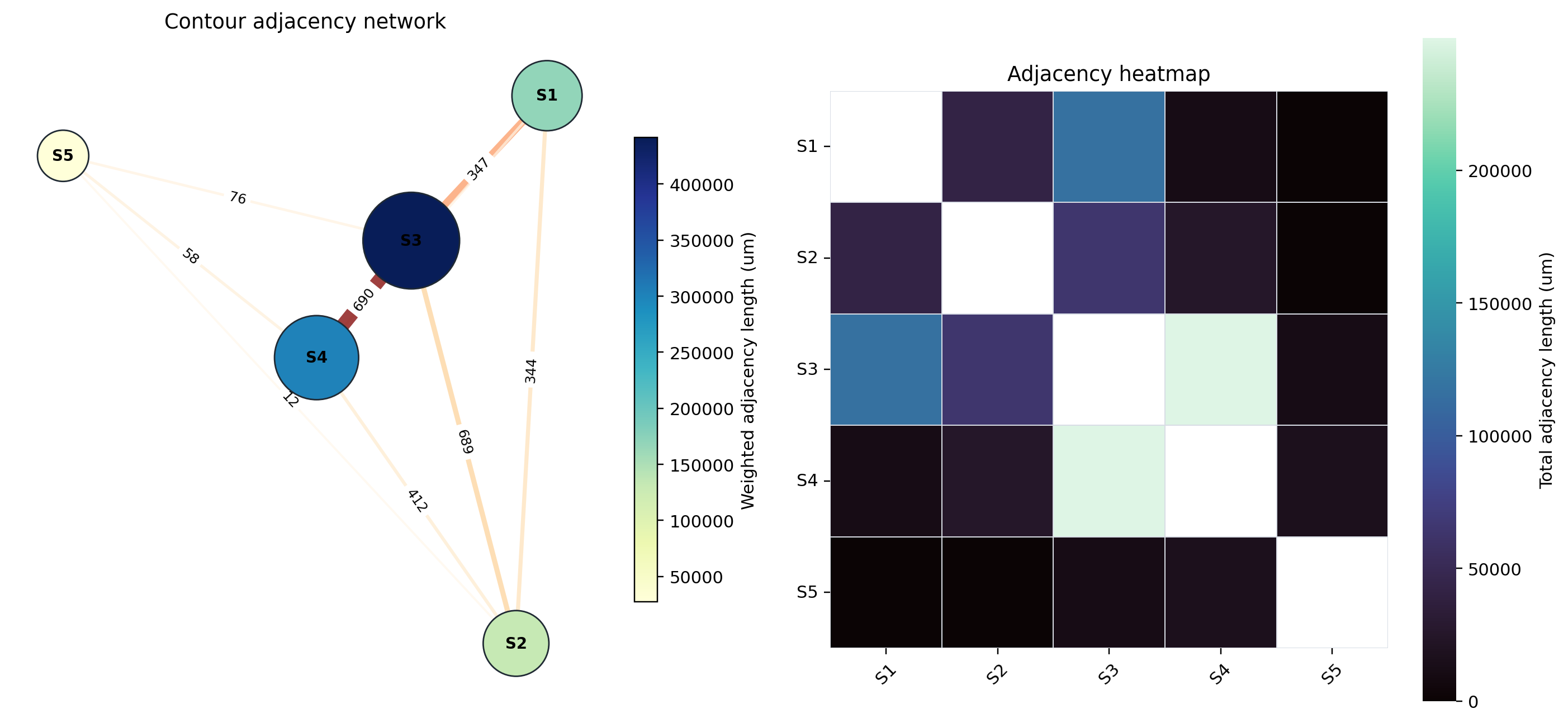
The network emphasizes the same geography seen in the table. S3 and S4 form the dominant adjacency axis (249809 um total adjacency), reflecting extensive contact between the myeloid-vascular-stromal niche and the myoepithelial/DCIS CAF/plasma compartment. S1 is most strongly connected to S3 (116321 um), supporting an invasive tumor/CAF boundary with vascular-myeloid stroma. S2 also contacts S3 (64381 um), while S5 is comparatively peripheral and has no direct positive adjacency with S1 in this S1-S5 contour export.

For reproducibility, the adjacency matrix in microns is:

	S1	S2	S3	S4	S5
S1	nan	41863	116321	10920.2	0
S2	41863	nan	64380.6	25296.1	554.3
S3	116321	64380.6	nan	249809	10917
S4	10920.2	25296.1	249809	nan	16172.5
S5	0	554.3	10917	16172.5	nan

9. Output files

The lightweight RTD snapshot uses these committed top-slice DEG artifacts plus the compact HistoSeg adjacency outputs:

• s1_s5_contour_counts.csv

• s1_s5_transcript_de_global.csv

• s1_s5_transcript_de_one_vs_rest.csv

• s1_s5_cell_composition_stats.csv

• s1_s4_s5_boundary_de_global_outward_0_60.csv

• s1_s4_s5_barrier_ring_density_top10.csv

• s1_s5_contour_adjacency_edges.csv

• s1_s5_contour_adjacency_matrix.csv

• s1_s5_contour_adjacency_metrics.json

• s1_s5_contour_adjacency_network.png

• s1_s5_contour_adjacency_heatmap.png

• s1_s5_contour_adjacency_overview.png

Local reruns also write full all-gene DEG tables and the full adjacency run directory under pyxenium_tutorial_outputs/atera_s1_s5_contour_application/ beside the Xenium export. Those full tables are intentionally not committed to the docs repository.