pyXenium.io Tutorial

Overview

This notebook uses the public 10x Genomics FFPE human renal carcinoma Xenium RNA + protein study to show how pyXenium.io preserves the structures that matter for downstream biology: cells, transcript points, aligned H&E, and cluster-aware metadata.

Biological question

Before we ask multimodal or topology questions, how do we keep the Xenium export organized enough to recover tissue architecture, image context, and molecular measurements in one reproducible container?

from __future__ import annotations

import json
import os
import sys
from pathlib import Path

import pandas as pd
from IPython.display import Image, Markdown, display


def find_repo_root() -> Path:
    for candidate in (Path.cwd(), *Path.cwd().parents):
        if (candidate / "pyproject.toml").exists():
            return candidate
    raise RuntimeError("Could not locate the pyXenium repository root.")


REPO_ROOT = find_repo_root()
SRC_ROOT = REPO_ROOT / "src"
if str(SRC_ROOT) not in sys.path:
    sys.path.insert(0, str(SRC_ROOT))

pd.set_option("display.max_columns", 20)
pd.set_option("display.max_rows", 12)

RENAL_DATASET_PATH = Path(
    os.environ.get(
        "PYXENIUM_RENAL_DATASET",
        r"Y:\long\10X_datasets\Xenium\Xenium_Renal\Xenium_V1_Human_Kidney_FFPE_Protein",
    )
)
SMOKE_ARTIFACT_DIR = REPO_ROOT / "manuscript" / "evidence" / "smoke_auto"
RUN_LIVE_IO_DEMO = RENAL_DATASET_PATH.exists()

RENAL_DATASET_PATH, SMOKE_ARTIFACT_DIR, RUN_LIVE_IO_DEMO

(WindowsPath('Y:/long/10X_datasets/Xenium/Xenium_Renal/Xenium_V1_Human_Kidney_FFPE_Protein'),
 WindowsPath('D:/GitHub/pyXenium/manuscript/evidence/smoke_auto'),
 True)

Dataset

• Raw study: 10x Genomics Xenium FFPE human renal cell carcinoma RNA + protein bundle.

• Versioned evidence in this repository: manuscript/evidence/smoke_auto/ and manuscript/figures/figure1_pyxenium_validation.png.

• Public surface used in this tutorial: read_xenium, read_slide, write_xenium, and export_xenium_to_slide_zarr.

Setup

The committed outputs below come from a real renal dataset run. The live demo cell also loads the local Xenium bundle when RENAL_DATASET_PATH exists.

smoke_payload = json.loads((SMOKE_ARTIFACT_DIR / "summary.json").read_text(encoding="utf-8"))
summary = smoke_payload["summary"]

core_summary = pd.DataFrame(
    {
        "metric": [
            "cells",
            "RNA features",
            "protein markers",
            "sparse nnz",
            "spatial coordinates",
            "cluster labels",
        ],
        "value": [
            summary["n_cells"],
            summary["n_rna_features"],
            summary["n_protein_markers"],
            summary["x_nnz"],
            summary["has_spatial"],
            summary["has_cluster"],
        ],
    }
)

display(core_summary)
display(pd.DataFrame(summary["largest_clusters"]).head(5))
display(pd.DataFrame(summary["top_protein_markers_by_mean_signal"]).head(5))

	metric	value
0	cells	465545
1	RNA features	405
2	protein markers	27
3	sparse nnz	16454170
4	spatial coordinates	True
5	cluster labels	True

	cluster	n_cells
0	1	87757
1	2	67261
2	3	59896
3	4	53975
4	5	35331

	marker	mean_signal	positive_cells
0	Vimentin	234.769989	455851
1	CD45	206.936478	446921
2	PTEN	149.335358	464946
3	CD3E	142.478271	285619
4	CD68	120.736671	244801

Core workflow

The canonical I/O path keeps Xenium data close to the original assay structure.

from pyXenium.io import (
    export_xenium_to_slide_zarr,
    read_slide,
    read_xenium,
    write_xenium,
)

slide = read_xenium(
    RENAL_DATASET_PATH,
    as_="slide",
    prefer="h5",
    include_transcripts=True,
    stream_transcripts=True,
    include_images=True,
)

payload = write_xenium(slide, "./renal_example.zarr", format="slide", overwrite=True)
reloaded = read_slide(payload["output_path"])
compat_store = export_xenium_to_slide_zarr(RENAL_DATASET_PATH, overwrite=True)

For the committed notebook output we execute only the loading step, because the full round-trip writes a large real-data store.

from pyXenium.io import read_xenium

if RUN_LIVE_IO_DEMO:
    slide = read_xenium(
        str(RENAL_DATASET_PATH),
        as_="slide",
        prefer="h5",
        include_transcripts=True,
        stream_transcripts=True,
        include_boundaries=False,
        include_images=True,
    )
    live_summary = pd.DataFrame(
        {
            "component": [
                "table cells",
                "RNA features",
                "protein markers",
                "streamed point layers",
                "image layers",
                "cluster key",
            ],
            "value": [
                int(slide.table.n_obs),
                int(slide.table.n_vars),
                int(slide.table.obsm["protein"].shape[1]),
                ", ".join(slide.component_summary()["points"]),
                ", ".join(slide.component_summary()["images"]),
                slide.metadata.get("cluster_key"),
            ],
        }
    )
    display(live_summary)
else:
    display(Markdown("Set `PYXENIUM_RENAL_DATASET` to a local renal Xenium bundle to run the live loading demo."))

	component	value
0	table cells	465545
1	RNA features	405
2	protein markers	27
3	streamed point layers	transcripts
4	image layers	he
5	cluster key	gene_expression_graphclust

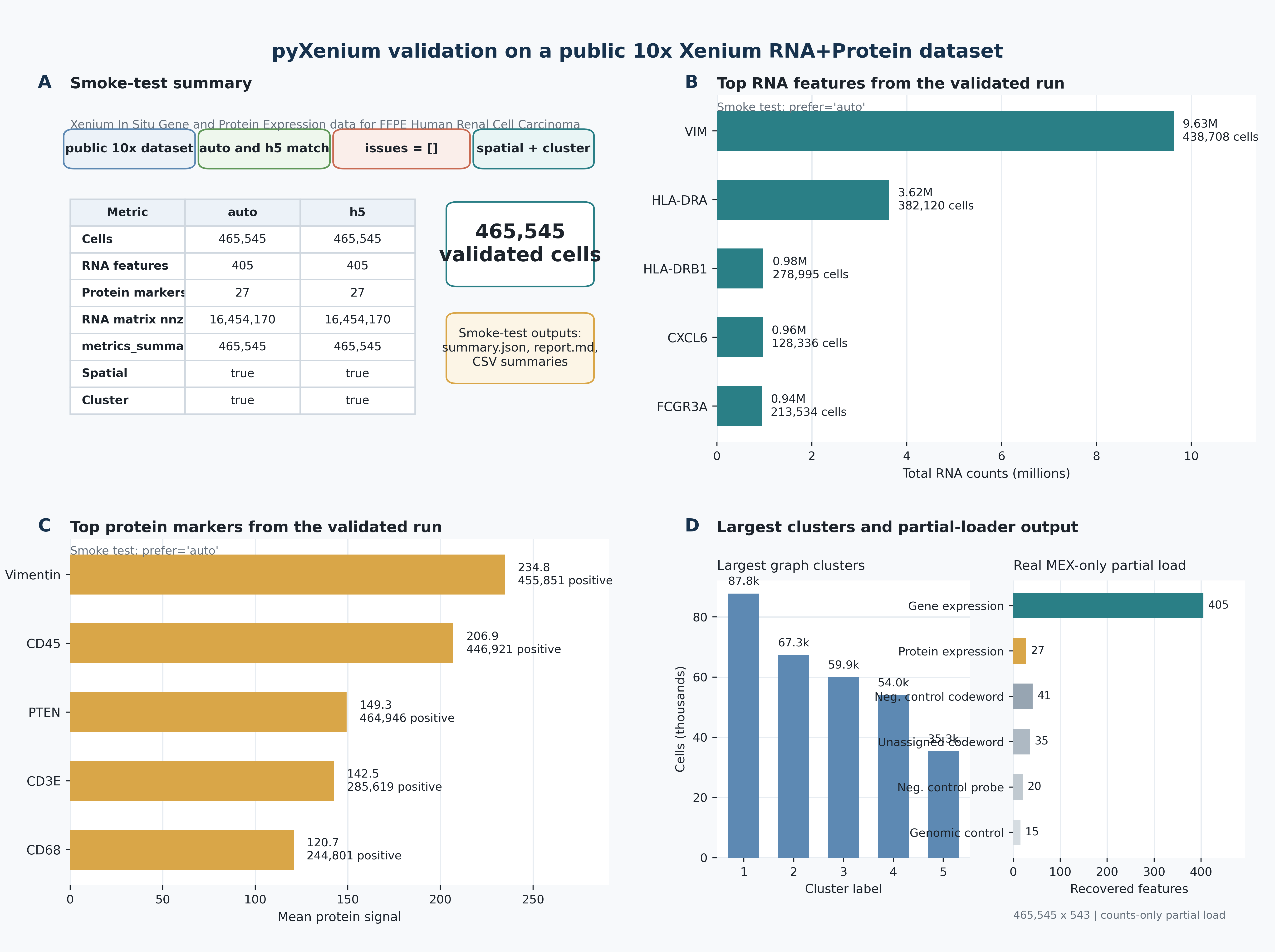
Visual outputs

The validation figure below summarizes the same renal study at the documentation level: loader checks, feature recovery, and multimodal readiness.

display(Image(filename=str(REPO_ROOT / "manuscript" / "figures" / "figure1_pyxenium_validation.png")))

Biological interpretation

For renal immune-resistance work, I/O is not a neutral preprocessing step. It decides whether we can later connect protein-dominant states, transcript neighborhoods, and histology-aligned niches back to the same tissue coordinates. The validated renal bundle shows that pyXenium keeps enough structure to recover 465,545 cells, 405 RNA features, 27 protein markers, and aligned image context without collapsing those layers into a lossy flat table.

Caveats

• The fully materialized round-trip examples are intentionally shown as code only because writing full real-data stores is much heavier than documentation rendering.

• This notebook streams transcript points instead of materializing them into memory; that is the preferred pattern for large Xenium exports.

• The public renal dataset is a validated reference, not a universal benchmark for every panel or tissue.

Next steps

• Continue into the multimodal notebook to see how this same renal study becomes joint state, discordance, and niche analysis.

• Use read_xenium(..., as_="slide") when you need images, shapes, or streamed transcripts together.

• Use load_rna_protein_anndata(...) when you are ready to work on joint RNA + protein analysis directly.